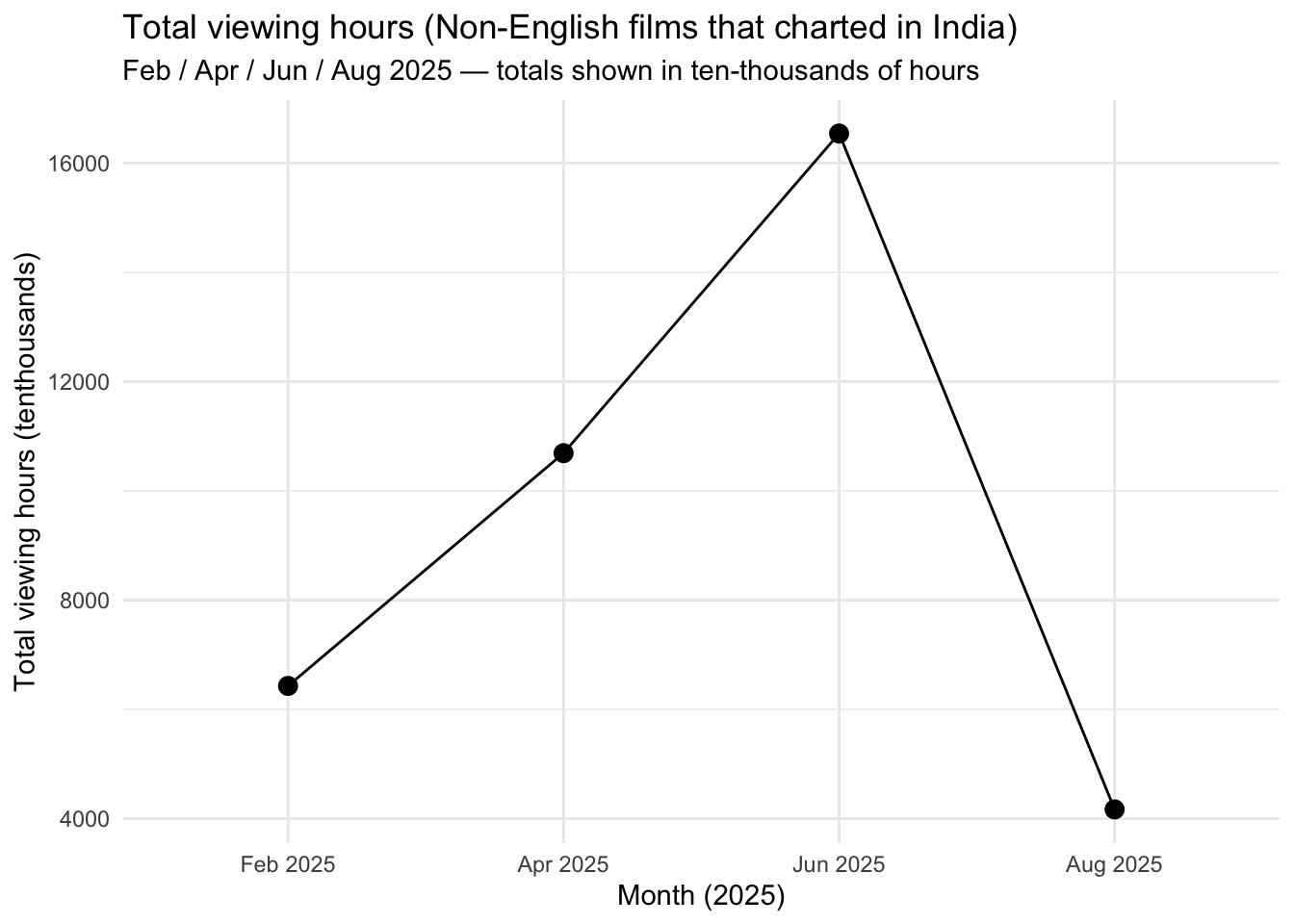
#We will take the top ten india data from the country dataset and
#use a few different months in 2025. this data will only include
#non-english top ten titles in india to assume that those are hindi. Now
#we will use this data to search up all these titles in the global #dataset.
#This will allow us to make a table that includes the #columns cummulative weeks in top ten,
#weekly_hours_viewed, runtime,
#and weekly hours viewed divided by runtime.
#We will also take an #average of the times
#watched column so that we can find the #estimated customer base

library(dplyr)
library(lubridate)
library(ggplot2)

months_to_do <- list(
  feb2025 = list(year = 2025, month = 2, label = "Feb 2025"),
  apr2025 = list(year = 2025, month = 4, label = "Apr 2025"),
  jun2025 = list(year = 2025, month = 6, label = "Jun 2025"),
  aug2025 = list(year = 2025, month = 8, label = "Aug 2025")
)

process_month <- function(year_i, month_i, label_i) {
  # India Top-10 titles for the month
  india_titles <- COUNTRY_TOP_10 |>
    filter(country_name == "India",
           year(week) == year_i,
           month(week) == month_i,
           weekly_rank <= 10) |>
    select(show_title) |>
    distinct()

  # Global rows for same month
  global_month <- GLOBAL_TOP_10 |>
    filter(year(week) == year_i, month(week) == month_i)

  # Keep only global rows that match India titles
  matched <- merge(india_titles, global_month, by = "show_title", all.x = FALSE, all.y = FALSE)

  # Keep non-English films only
  matched_noneng <- matched |>
    filter(category == "Films (Non-English)")

  if (nrow(matched_noneng) == 0) {
    return(tibble(
      month = character(0),
      show_title = character(0),
      cumulative_weeks_in_top_10 = numeric(0),
      month_hours = numeric(0),
      runtime = numeric(0),
      est_views = numeric(0)
    ))
  }

# Summarize per title, I assumed that the non-english films would be hindi and
# I also assumed and filtered out movies with runtimes shorter than 1.8
#  based on cultural contextt, most hindi
#  films have runtimes over 1.75, whereas most westerns ones do not.
  matched_noneng |>
    group_by(show_title) |>
    summarize(
      cumulative_weeks_in_top_10 = max(cumulative_weeks_in_top_10, na.rm = TRUE),
      month_hours = sum(weekly_hours_viewed, na.rm = TRUE),
      runtime = if (all(is.na(runtime))) NA_real_ else first(runtime[!is.na(runtime)]),
      .groups = "drop"
    ) |>
    filter(!is.na(runtime), runtime >= 1.8) |>
    mutate(
      est_views = round(month_hours / runtime),
      month = label_i
    ) |>
    select(month, show_title, cumulative_weeks_in_top_10, month_hours, runtime, est_views) |>
    arrange(desc(month_hours))
}

# run for each month and combine
results_list <- lapply(months_to_do, function(m) process_month(m$year, m$month, m$label))
combined_tbl <- bind_rows(results_list)